Chapter 1 - VCF file to GWAS matrix • VCFtoGWAS

If you have access to the Rmarkdown files, you’ll find the files for this chapter here

Step 1.1 - Upload VCF to R

This step mainly uses the “Upload_vcf_to_R” function. Description can also be seen by running ?Upload_vcf_to_R in the console of Rstudio after loading the VCFtoGWAS package.

Steps:

Load VCFtoGWAS library
Define parameters used for uploading and saving:
- VCF file path
- Path where you wish to save your results
- Whether you’d like to save and/or see the results
Run Upload_vcf_to_R

What is returned is a list containing a filtered fixed section and a gt section with only the genotypes (see VCF info in General Section) and also the path where the two were saved (they’ll be used in the next step)

Output:

Notice that the “unwanted” column marks a strain that isn’t wanted (no pre-filtration was done). It can be omitted in the next step.

Step 1.2 - Filter

After extracting the fixed information and the gt section from the vcf file, it is time to filter the data.

First of all, if the uploaded vcf wasn’t pre-filtered to contain only the desired strains (by using the “usegalaxy” VCFselectsamples tool), you can use this step to get only the strains that you wish to analyze. If an array of strain names isn’t provided, all the strains in the file will be used for further analysis.

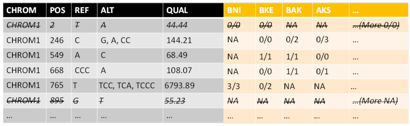
After filtration, some rows (SNPs) might not contain any data at all (all NA). So the second thing that is done in this step is omitting those variants (SNPs).

Notice that you can choose whether or not to omit SNPs that are known to not appear in any of the remaining population. Meaning the information exists but they don’t appear in any strain. The reason to filter is that the amount of examined SNPs affects the p-values after correcting for multiple testing. The reason to not filter is that they are sort of a baseline and maybe shouldn’t be omitted. I decided to filter.

For example, for the 60 strains I worked on, the initial amount of variants is: 1,754,866

After filtering only by “all NA”, the amount was reduced to: 1,754,079 (meaning 787 were omitted)

But after filtering by “all [NA and/or 0/0]”, the amount was reduced to: 393,334 (meaning 1,361,532 were omitted). The latter was what I used in my tests.

The main function used in this step is the “Filter_genotypes”.

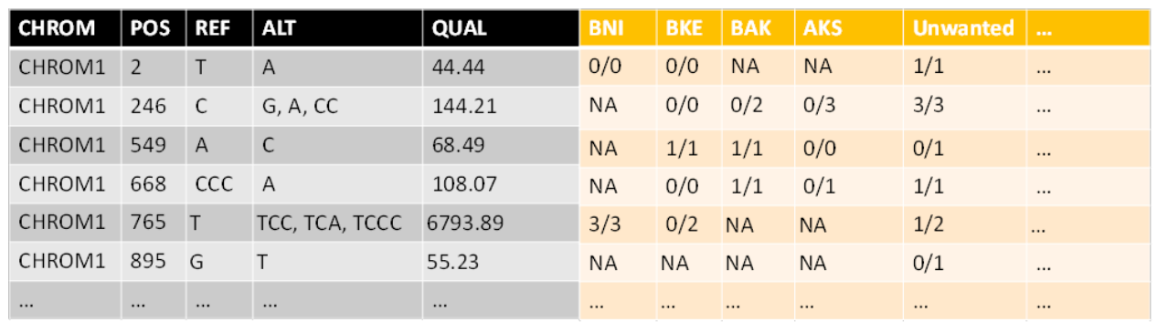
The function returns a list of 3 objects: the fixed information (the left part of the output illustration), the filtered genotype matrix (the right part), and a string of the directory where the file are saved.

Output:

Notice that the “unwanted” column was filtered out. Also the last row that contained all Na. If you chose to keep rows with SNPs that are 0/0 across all strains, the first row will not be omitted

Step 1.3 - Expand

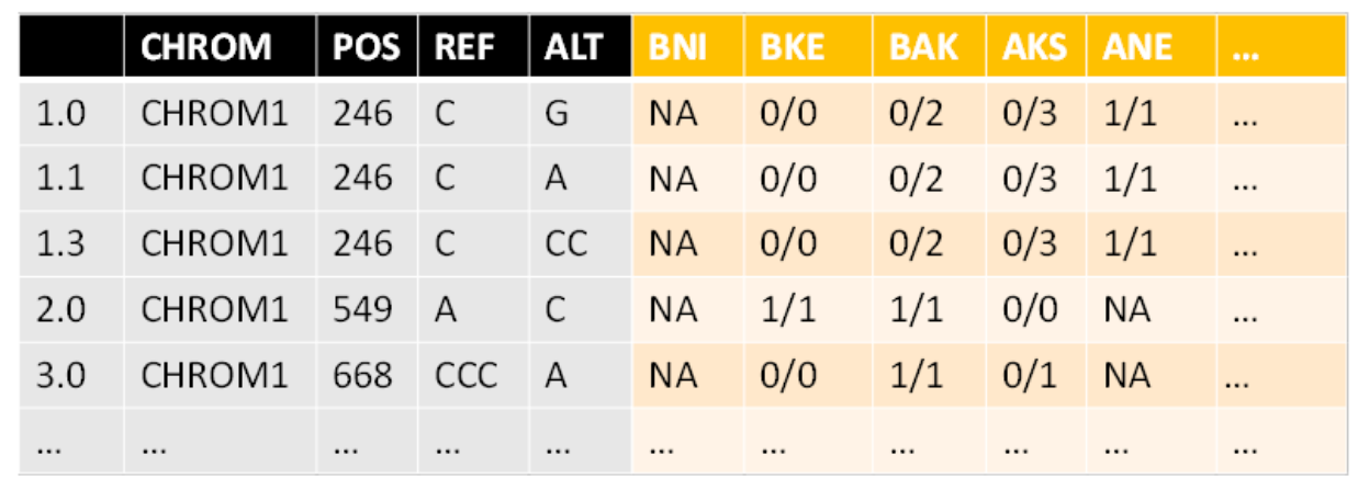
In this step, the fixed info (the left part of the output illustration) is expanded so that each row will represent only one SNP or INDEL and not multiple options per position. The genotype matrix is equally expanded.

In other words, the aim now is to make each row SNP-specific rather than location-specific. The number of variants (alterations) per chromosomal location is saved in an array named “indication”.

Before expanding, the fixed info looks like this:

        CHROM POS REF  ALT 
1 chromosome1  33  CA    C 
2 chromosome1 137   C  CCT 
3 chromosome1 176  CG C,AG 
4 chromosome1 184   C    G

Then after expanding:

          CHROM POS REF ALT 
1.0 chromosome1  33  CA   C 
2.0 chromosome1 137   C CCT 
3.0 chromosome1 176  CG   C 
3.1 chromosome1 176  CG  AG 
4.0 chromosome1 184   C   G

In this case, the indication array will be: c(1, 1, 1, 2, 1)

As for the genotype matrix, we replicate rows similarly to how they were replicated in the fixed information:

Going from:

                CCG   BNT   BHF CEQ   CFR   BQQ   
chromosome1_33  NA    NA    NA  NA    NA    "0/0" 
chromosome1_137 NA    NA    NA  "0/0" NA    NA    
chromosome1_176 "0/1" "0/0" NA  "0/2" "0/0" NA    
chromosome1_184 "0/1" "0/0" NA  NA    "0/0" "0/0"

To:

                  CCG   BNT   BHF CEQ   CFR   BQQ   
chromosome1_33    NA    NA    NA  NA    NA    "0/0" 
chromosome1_137   NA    NA    NA  "0/0" NA    NA    
chromosome1_176   "0/1" "0/0" NA  "0/2" "0/0" NA    
chromosome1_176.1 "0/1" "0/0" NA  "0/2" "0/0" NA    
chromosome1_184   "0/1" "0/0" NA  NA    "0/0" "0/0"

The indication array will help us in the next step. You can see in the expanded example above that rows 3 and 4 are identical for the genotype matrix (chr1_176 and chr1_176.1) but are different for the fixed info (3.0 and 3.1).

So, when creating the GWAS matrix, we use the indication array to know which digit to look for. The 3rd index in the array is “1”, so in row number 3 in the genotype matrix, we count the number of instances of the number “1” for each strain (0/1 is 1 instance, 1/1 is 2 instances, 0/0 is 0 instances and so is 0/2). The 4th index in the array is “2”, so in row number 4 in the genotype matrix, we count the number of instances of the number “2” for each strain (0/2 is 1 instance…).

The main function used here is “Expand_files”

Output:

Notice that now every row has one REF and one ALT.

Step 1.4 - Create GWAS Matrix

In this step, a GWAS matrix will be created and with this the first chapter of the process ends¹.

You can choose if you want the matrix to include only SNPs or SNPs and INDELs (default is both SNPs and INDELs) Also, after expanding in the previous step, some variants are now all 0/0 so we need to take those out now.

In this step, we go row by row, and by using the indication array from the previous step we determine the value given for each [i, j] element in the genotype matrix. The value can be 0, 1, 2 or NA. If we refer to the allele containing the SNP as the minor allele and we use the classic genetics nomenclature then a value of 0 is “A/A”, 1 is “a/A” and 2 is “a/a”. (a/a means a SNP appears in both alleles of strain)

The main function used in this step is “Get_GWAS_matrix”.

Output:

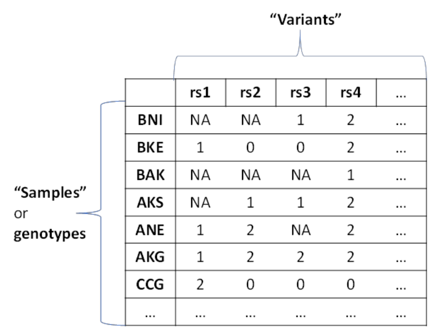
The output consists of a matrix that can be used for the GWAS analysis and also the mapping information (what was the fixed info until now) which is also needed for the analysis.

Notice that until now the genotypes (strains) were column names but are now row names.

GWAS matrix: _{(rs = reference SNP)}

Step 1.5 - Offspring GWAS matrix

Once a GWAS matrix for the parents was constructed, a matrix for the offspring can be constructed:

Let’s look at two possible parents and 6 snps (covering all the possibilities). The 3rd row shows the offspring of these parents and the value options for these snps for it. The 4th row shows the probability for each value option to happen (given the specific situation).

For example, for rs4 - both parents are 1 (“A/a”) and therefore the probability for the offspring to be 1 (“A/a”) is 0.5, to be 0 (“A/A”) is 0.25 and to be 2 (“a/a”) is 0.25.

	rs1	rs2	rs3	rs4	rs5	rs6
BHF	0	0	0	1	1	2
CEQ	0	1	2	1	2	2
BHFCEQ	0	0/1	1	0/1/2	1/2	2
Prob.	1	\(\frac{1}{2}\)/\(\frac{1}{2}\)	1	\(\frac{1}{4}\)/\(\frac{1}{2}\)/\(\frac{1}{4}\)	\(\frac{1}{2}\)/\(\frac{1}{2}\)	1

In this manner the offspring GWAS matrix is built.

Note: If either parent has missing info for a SNP (NA), the offspring will also get NA